Statistics

SAT SUMX = 5846, SUMX^2 = 3428148

A) Mean = 5846 / 10 = 584.6

B) S = ((SUMX^2-(((SUMX)^2)/N))/(N-1))^.5

   S = ((3428148-(((5846)^2)/10))/(10-1))^.5

   S = ((3428148-3417571.6)/9)^.5

   S = 1175.12^.5

   S = 34.28

C) 95%CI = +- t(.05)SsubXBAR + XBAR

   SSubXBAR = (s)/(n^.5) = 34.28/3.16 = 10.85

   95%CI = +- t(.05)10.85 + 584.6 = +-(2.2622*10.85)+ 584.6

   95%CI = 560.07 - 609.13 or the whole scores of 560-609.  542 is not in the expected range of the population mean, thus the course has a statistical significance of improving the scores.

By using a confidence interval of 95%, we can be 95% sure that the population mean is contained within 560.06 - 609.14.   Since a mean of 542 is not within this range, we have can conclude that the new course did indeed improve the SAT verbal scores.

By performing a one-tailed t test we can analyze this:

Set H0: u0<=u

Set H1: u>u0

in plain language:  our null hypothesis is that the sample mean is equal to or less than the population mean.  Our alternative hypothesis is that the sample mean is greater than the population mean.

t = (584.6-542)/(10.841) = 3.93

t(.01),df=9 = 2.82, p<.01

Rejection Rule:   For H1:m > m0, reject H0 if tcomp > tcrit 

We reject H0.

The new course did improved the SAT verbal scores

Question #2

                                                  Descriptive Statistics

Our Null hypothesis:  H0 = u1 - u2 = 0 (there is no difference in the scores of the yellow group and green group)

Our alpha level is .05, we are looking for a 95% CI

Since N is different for each group, we use the formula: 

s sub Xbar sub 1 minus X bar sub 2 = ((((N1-1)(s2sub1) + (N2-1)(S2sub2))/(N1+N2-2))((1/N1)+(1/N2)))^.5

OR: (s2pooled(1/N1 + 1/N2))^.5 

S2sub1 = 19.3

S2sub2 = 146.25

N1=5

N2=4

So we get: s2pooled = ((4*19.3)+(3*146.25))/7

s2pooled = 515.95/7 = 73.71

s sub Xbar sub 1 minus X bar sub 2 = (73.71(1/5 + 1/4))^.5 = 5.76, or the standard error difference

Now find t sub xbar sub 1 minus xbar sub 2 = (Xbar1 - Xbar2)/s sub Xbar sub 1 minus X bar sub 2

=20.60-29.25/5.76 = -1.50

Using table B, we find a critical value for T where df = N1+N2-2, or 7

Using the 5% level for t(.05) we get 2.36

Rejection Rule:  Reject H0 if |tcomp| >= tcrit

|tcomp| = 1.5 which is less than 2.36, or tcrit, therefore we do not reject H0, meaning that we cannot conclude the yellow paper caused subjects to score lower.  The answer is no

T-Test, Question 2

                                                      Group Statistics

Independent Samples Test

Equal variances assumed

Question #3                         Statistics

a  Multiple modes exist. The smallest value is shown

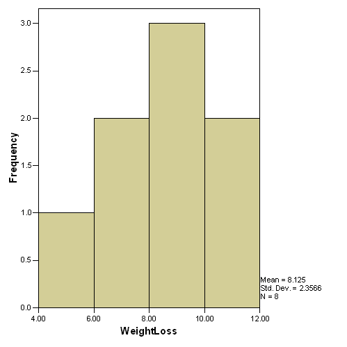
For Diet A, the most appropriate descriptive statistic is the mean.  Since multiple modes exist, the mode is not very useful.  The median is slightly lower than the mean, giving it a slight positive skew, hence the mean is the most useful.

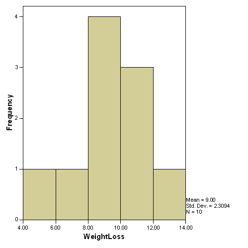
For Diet B, the median, mean and mode are all equal, hence all useful.

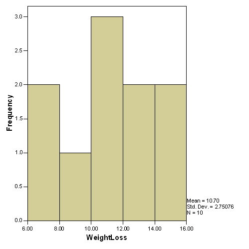
For Diet C, there is a slight negative skew.  Multiple modes exist, so the mode is not useful.  Because the skew is only slight, the mean is the most useful.

Histograms are the best graphs for these diets.

Graph of Diet A

Diet B

Diet C

#3, Oneway ANOVA

Build a matrix of values based on the data for Diet A, Diet B, Diet C

Ho: m1 = m2 = m3         

Ha: At least one mean differs from the others.   

Rejection Rule:  Reject Ho if p-value < .05       

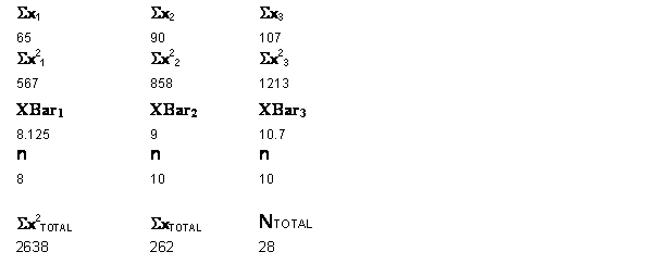          SPSS ANOVA

Weight_Loss

P value = .099 > .05 --> Accept H0.

F(2,25) = 3.39 , p = .099

There is no significant difference in mean wieght loss among the different diets

#3 b) Post Hoc Tests

                                                                                  Multiple Comparisons

Dependent Variable: Weight_Loss

LSD

*  The mean difference is significant at the .05 level.

There was a significant difference between Diet A and Diet C

#3 b) A graph of the means

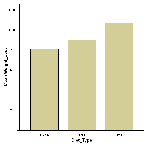
#4, Two Way ANOVA, Type I Sum of Squares

F(1,22)=0.006, p>.05

There is no significant population mean difference among Gender

F(2,22)=6.872, p<.01

There is a significant population mean difference in the diets

F(2,22)=3.598, p<.05

There is a significant interaction between diets and gender

                                                     Tests of Between-Subjects Effects

Dependent Variable: Weight_Loss

a  R Squared = .488 (Adjusted R Squared = .371)

Because problem #4 contains different values of n for each group, the Type III sum of squares as computed in SPSS does not match the manual sweep-matrix as taught in class.  So I used a Type I sum of squares (highlighted) which more closely resembles the manual calculations.

I am including the TYPE III SPSS mean of squares results for this question below, with different answers due to the different results of the same data, neither of which matches manual computations:

                                                      Tests of Between-Subjects Effects

Dependent Variable: Weight_Loss

a  R Squared = .488 (Adjusted R Squared = .371)

F(1,22)=0.685, p>.05

There is no significant population mean difference among Gender

F(2,22)=8.155, p<.01

There is a significant population mean difference in the diets

F(2,22)=3.114, p>.05

There is no significant interaction between diets and gender

LSD TEST, POST HOC

                                                                           Pairwise Comparisons

Dependent Variable: Weight_Loss

Based on estimated marginal means

a  Adjustment for multiple comparisons: Least Significant Difference (equivalent to no adjustments).

There is no significant mean difference between Gender

                                                                     Pairwise Comparisons

Dependent Variable: Weight_Loss

Based on estimated marginal means

*  The mean difference is significant at the .05 level.

a  Adjustment for multiple comparisons: Least Significant Difference (equivalent to no adjustments).

There is no significant difference between Diet A and Diet B

There is a significant difference between Diet A and Diet C

There is a significant difference between Diet C and Diet B

Dependent Variable: Time

a  R Squared = .835 (Adjusted R Squared = .786)